Advanced Algorithm Project
1. INTRODUCTION
The minimum vertex cover problem belongs to the class NP-hard with numerous applications in computational biology; it is intractable to search for an optimal solution. We will implement three algorithms: branch and bound with heuristic approximation guarantee, hill climbing, and simulated annealing, in order to search for a near-optimizated solution by evaluating each algorithm theoretically and experimentally.
The branch and bound algorithm is designed using Depth First Search rather than Breadth First Search, and the heuristic approximation selected is a 2-approximation algorithm that chooses any remaining edges in the graph. Theoretically and experimentally, this has a high time-complexity but can obtain a global optimal solution given enough time. We will change the searching method from BFS to DFS for two reasons. One, it gives a considerable solution as well as an upper bound first. This helps to limit the size of the priority queue and get considerable solutions for execution. Second, this limits the increase in size of the priority queue to avoid stack overflow.
Hill climbing is a form of local search. We start by keeping all vertex in a large vertex cover, and continuously try to remove the vertex with the smallest degree until we are unable to maintain a vertex cover. The implementation involves an ordering of the vertex by degree in ascending order and trying to remove vertex with the lowest degree at each iteration. The algorithm performs well experimentally with just a slight percentage error from the optimal solution and an acceptable running time.
Simulated annealing is another form of local search. Similar to hill climbing, but it adds a mechanism that can jump out of local minimum by accepting a worse solution based on a probability. This makes it more likely to reach the global optimal solution. Overall the algorithm performs efficiently with relatively low error.
2. RELATED WORK
There are numerous algorithms for solving the minimum vertex cover problem efficiently. The fastest solutions utilize the heuristic approximation algorithms; they can usually provide near-optimal solutions within polynomial time. Some local search algorithms like the genetic algorithm, hill climbing and simulated annealing can also obtain near-optimal solutions as compared to heuristic approximation guarantees. Meanwhile, a high complexity branch and bound algorithm can find the global optimal solution in exponential time.
3. ALGORITHMS
3.1 Branch and bound
The branch and bound algorithm starts with an empty set of vertex, an initial upper bound equal to the number of vertex in the graph, and an empty priority queue to store any unsolved subproblems ordered by their lower bounds. For every branch, we choose the vertex with the highest degree in current graph and expand the problem into two new subproblems that collect either the vertex or all its neighbors into the vertex cover and update the graph respectively. Then we use a heuristic approximation algorithm to calculate the lower bound for each subproblem. If the lower bound does not exceed the upper bound, we put the subproblem with a larger lower bound into the priority queue. We then move on using the subproblem with a smaller lower bound, and repeat. If the solution is better than the upper bound, we update the upper bound and the current best vertex cover as the subproblem, else we just keep the current best vertex cover and upper bound. Then we pop the next subproblem in the priority queue and continue the process until the priority queue is empty or the next subproblem’s lower bound is larger than the upper bound (a new best). This means all remaining subproblems would give a solution larger than the current best solution, thus the current best solution is the global optimal solution.
Below is the pseudo-code for our branch and bound implementation:1
2
3
4
5
6
7
8
9
10
11Initialize PriorityQueue Q;
Initialize Best;
Put an empty element into Q;
while (!Q.isEmpty()) {
curVC = Q.remove( );
dupG = duplicate the original graph G;
curG = cut the dupG based on curVC;
temp = DFS(curVC,curG);
if (temp < Best)
Best=temp;
}
And the DFS function is:1
2
3
4
5
6
7
8
9
10
11
12
13
14while (!curG.adj.isEmpty()) {
nextV = nextV(curG);
curVC2 = duplicate curVC;
add nextV into curVC;
add all its neighbors into curVC2;
LB1 = approx(nextV,curG);
LB2 = approx(neighbors of nextV,curG);
if (both of them are smaller than Best)
put larger lowerbound into Q,continue;
if (one of them is smaller than Best)
continue that one;
if (both of them are larger than Best)
break;
}
In this algorithm, the calculation of lower bound uses the approximation guarantee and we would talk about it in next section. Also we implement some useful functions for getting a more precise solution. The pseudo-code are listed below.1
2
3
4
5
6
7
8
9
10
11
12
13
14
15
16
17
18
19int nextV(Graph G) {
initialize nextV = 0;
for i = one vertex of G
if i has more neighbors,update nextV;
return nextV;
}
Graph dupG(Graph G) {
Hashtable<>dupG=new Hashtable<>();
for each edge in G
duplicate it into dupG;
return new Graph(dupG);
}
Graph restG(List curVC,Graph G) {
Set restV=G.vertex
restV.removeAll(curVC);
while(restV is not empty) {
remove vertex in G;
}
}
Theoretically, this algorithm has a high time and space complexity. Since we need to store all subproblems in a priority queue, the length of the queue can be, in worst case, the number of vertex in graph where each element is a set of vertex (a list of chosen vertex numbers), consequently worsening the space complexity. Since the algorithm never stops before the queue is empty or the lower bound of next subproblem is larger than the current best solution, the time complexity for the loop – in the worst case – is equal to the max number of subproblems. Within each iteration, we provided some tools to find the vertex with the highest degree, duplicate the graph, cut the graph, and find the approximation guarantee. Since all these functions are in polynomial time, the total time complexity is polynomial as well.
The time and space complexity for this algorithm is theoretically high. Since we need to store all subproblems in priority queue, the length of the queue can be 2^n in worst case where n represents the number of vertex in graph while each elements in the queue is a set of vertex (a list of chosen vertex NO.), which would make the space complexity worse. While since the algorithm never stops before the queue is empty or the lower bound of next subproblem is larger than the best solution, the time complexity for the loop would be O(2^n) in worst case. And in each iteration, we provide some tools to find the vertex with the most degree, duplicate the graph, cut the graph and the approximation guarantee. Since all these functions are in polynomial time, the total time complexity would be O(2^n).
We see that the branch and bound algorithm can obtain the optimal solution given enough time. However it may waste resources if implemented without a timeout. We take the required amount of time into consideration and evolve the branch and bound algorithm so that it can provide the current best solution within an alloted amount of time.
3.2 Heuristics with approximation guarantees
The heuristic approximation guarantee is used for the branch and bound algorithm to calculate the lower bound of subproblems. We selected the 2-approximation algorithm introduced in the course. Below is the pseudo-code:1
2
3
4
5
6
7
8
9approx(List curVC,Graph G) {
Set restV=G.vertex;
restV.removeAll(curVC);
while(!restV.isEmpty()) {
get i from restV;
find i and one neighbor in G called j;
remove i,j and all neighbors in restV;
}
}
The algorithm is used to search for a solution at most 2 times worse than the optimal solution for minimum vertex cover. It starts with an empty vertex cover and a graph for searching. It randomly select any remain edge in the graph and collects both vertex of that edge into the vertex cover. The algorithm would stop when there are no more edges in the graph. This solution is larger than or equal to the optimal solution, otherwise it would contradict the initial assumption that we already have the size of the optimal solution. And this solution must be less than or equal to twice the size of optimal solution since this ensures all edges are covered by a set of vertex by using the edges themselves; at worst we have a set with size double the set of edges. The correctness of this algorithm has been proved in lecture.
As described in the lecture, the 2-approximation algorithm guarantees that the approximation lies between the size of the optimal solution and twice the size of the optimal solution. OPT≤APX≤2OPT. Based on that, the lower bound can be half the approximation 1/2APX.
Since all it needs to do is remove edges in the graph, in worst case the time complexity is equal to the number of edges in the graph O(E). The space complexity depends on the user reqirement: if the user wants to get just the size of the vertex cover, it doesn’t require extra space. If the user wants the exact vertex cover, it requires O(V) in worst case.
This heuristic algorithm benefits from an apparant polynomial time and space complexity, but suffers from the unprecise solution.
With research we found many other heuristic approximation algorithm with more precise solutions described in various papers. But for this task, the approximation is used only for the calculation of the lower bound, so the algorithm with a definite, lower time complexity would be benefit, thus we chose this algorithm.
3.3 Hill climbing
Starting from the whole set of vertex as the initial vertex cover, the only task of our hill climbing algorithm is to delete. Put simply, the algorithm keeps trying to delete one node from the current set each time, forming a new valid set whose size is one or more nodes smaller, until deletion of any node will result a an invalid vertex cover. The neighborhood in this case is defined as sets of nodes that are all one node smaller than the current.
The deletion order is based on a priority queue of node degree. The algorithm deletes the node with the smallest degree in the current solution (or more precisely, the priority queue), since it covers least number of edges. This approach can make the algorithm find a solution faster. If deletion of that node still results in a valid vertex cover, the algorithm will simply repeat. If the deletion is unsuccessful, meaning the remaining nodes can’t cover all edges, it indicates the node just picked is essential to the vertex cover. So, to always keep a valid vertex cover as the solution, the node must be added back to the solution, and the algorithm will continue to search and delete the next node with the smallest degree besides the one(s) just attempted.
If nodes have been examined and are deemed essential, they are also essential to smaller vertex covers found later, and needn’t be examined again. This is because if some edge(s) are only covered by one node in a partial solution, then in a smaller neighboring solution the edge(s) are still only covered by the same node. Deletion of this node will result in the uncovered edge(s). For this reason, each node in the graph only need to be examined once and subsequently removed from the priority queue, whether it was deleted or not.
Another case to consider is when several nodes have the same degree: the algorithm will take all nodes with the same degree and random choose an order to examine them in. This prevents the algorithm from getting stuck in the same local minima.
The algorithm ends when deletion of any node will result in an invalid vertex cover. In other words, it will end when the priority queue is empty. This will guarantee a local optimal solution because if there is smaller neighboring solution, the algorithm will find and reach it via deleting node(s), obtaining a smaller vertex cover.
Since the processing order of this algorithm is dependent on the degree of nodes, it is a relatively fixed one. The random step occurs when there are several nodes with same degree, making it easy to get stuck in some local minima, though it can obtain a local optimal solution faster than other algorithms.
Another similar approach is to select nodes randomly instead of choosing the node with the smallest degree. The running time remains the same, but percentage error is relatively large, thus this approach is discarded.1
2
3
4
5
6
7
8
9
10
11
12
13
14
15
16G ¬ graph;
vc ¬ the whole vertex;
pq ¬ the whole vertex with least degree priority;
while (pq.size != 0 && time < cutoff time)
list ¬ node with the same least degree removed from pq;
while (list.size() != 0)
nd ¬ pick and delete random one element in list;
delete nd from vc;
if (checkValidVertecCover(vc))
continue;
else
add nd back to vc;
endif
endwhile
endwhile
return vc;
3.4 Simulated annealing
The Hill Climbing deletes vertex in every iteration. So there is possible that one vertex in optimal solution is deleted in the early stage and then it’s stuck in local minimum. In order to fix this problem, Simulated Annealing is able to add back vertex back into the vertex cover based on a probability. The algorithm works as followed.
The initial vertex cover is all nodes.
Set an initial temperature and an end temperature. In every iteration, decrease the temperature by a small ratio.
In every iteration, randomly choose a vertex from original graph, There are two cases. First, if this vertex is already in vertex cover, delete it and check if the vertex cover is valid. If it’s still valid, which means deleting the vertex gets a smaller size vertex cover, so the algorithm accepts the new better vertex cover. if it’s not valid, add this node back to vertex cover to keep the vertex cover valid all the time. Second case is, if the randomly selected vertex is not in vertex cover, then add it to vertex cover. The vertex cover is still valid but it’s one more vertex larger, which means it’s a worse solution. However, maybe this vertex is just the vertex that may cause the Hill Climbing stuck into the local minimum. Therefore, the algorithm tries to accept this worse solution based on a probability p. We define p as p = exp( - ( 1 + deg(v) ) / temperature). Using this definition p is in range of 0 to 1 so we compare p to a random value between 0 to 1. If p is larger than this random value, accept the worse solution. If not, roll back.
The reason simulated annealing uses a probability is that it’s a good criteria. At early stage, almost all the vertices are in vertex cover, and the randomly selection process is very likely to pick and delete a vertex which is in optimal solution. Under such circumstances, the probability p is relatively close to 1 at early stage, which means it’s very likely to add back a vertex into vertex cover. Since temperature is decreasing in every iteration, the probability is also decreasing, the chance of adding back a vertex is decreasing.
The simulated annealing algorithm still is not guaranteed to return the optimal solution. But by setting a probability to add back vertex, it’s able to jump out of the local minimum and get close to the optimal solution.1
2
3
4
5
6
7
8
9
10
11
12
13
14
15
16
17
18
19
20G ¬ graph;
vc ¬ the whole vertex;
E ¬ end temperature;
alpha ¬ temperature decrease ratio;
while (temperature>E)
v ¬ radomly select one vertex;
while (v in vc )
delete v from vc
if (!checkValidVertecCover(vc))
add v back to vc;
else
add v into vc
endif
p = exp( - ( 1 + deg(v) ) / temperature)
if (p< RandomValueBetween01)
delete v from vc;
endif
endwhile
endwhile
return vc;
4. EMPIRICAL EVALUATION
4.1 Platform
Testing machine runs Windows 10 with a CPU Intel(R) Core™ i7-4710HQ CPU @ 2.50GHz, 8.00 GB RAM. The programming language we choose is Java with Java JDK 1.8.0.65 and the compiler to be JRE 1.8.
4.2 Evaluation criteria
4.2.1 Running Time
In this paper, our implementations includes a timeout that we based on theoretical runtimes and narrowed the range with experimental runtimes. As a compartor between algorithms, runtimes tells us about the algorithm’s efficiency, as well as provide a ruler for mearsuring the effects of various factors on efficiency, such as the size of the set of vertex or edge.
4.2.2 Relative Error
Besides running time, the accuracy of the algorithm greatly affects its usage and implementation. Multiples times we have iterated through an algorithm implementation due to the tradeoff between running time and accuracy. Relative error gives us another criteria to judge the algorithm implementation, such as checking whether or not increasing sample sizes affects accuracy. However, this measurement must be taken with a grain of salt, as local search algorithms often afford an element of randomness, thus we must be careful and take the average of numerous runs when recording data.
4.3 Obtained results
4.3.1 Comprehensive table
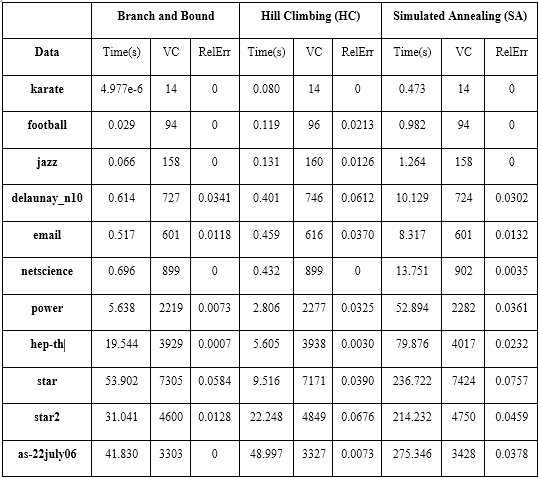
Table below shows the comprehensive information for the three algorithms respectively. The running time is in unit s, VC is the minimum vertex cover solution generated by algorithms within the running time, and the RelErr is the relative error which is calculated by the equation (SOLUTION-OPT)/OPT.
4.3.2 Approximation lower bound
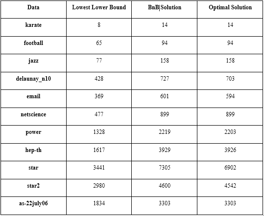
The next table shows the relation of the lowest lower bound generated by the heuristic approximation guarantee comparing with the solution of the branch and bound algorithm and the optimal one. The data in the table shows that for the lower bound task, the approximation algorithm do not need to give a better solution, since it always lower than the optimal solution. Meanwhile, the running time of the approximation algorithm do affect the time complexity of the branch and bound algorithm. So, instead of a precise algorithm, the approximation should choose a fastest one for a better performance of Branch and Bound.
4.3.3 QRTD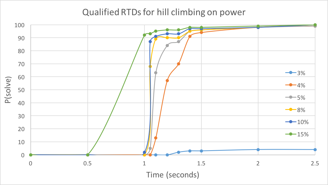
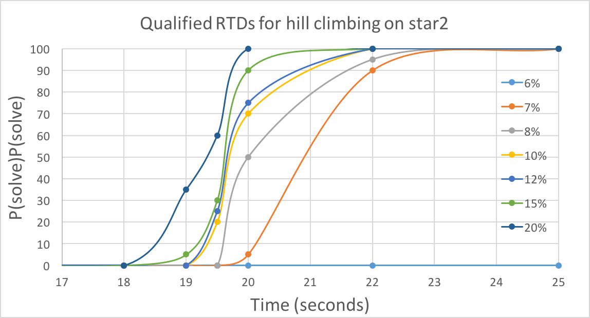
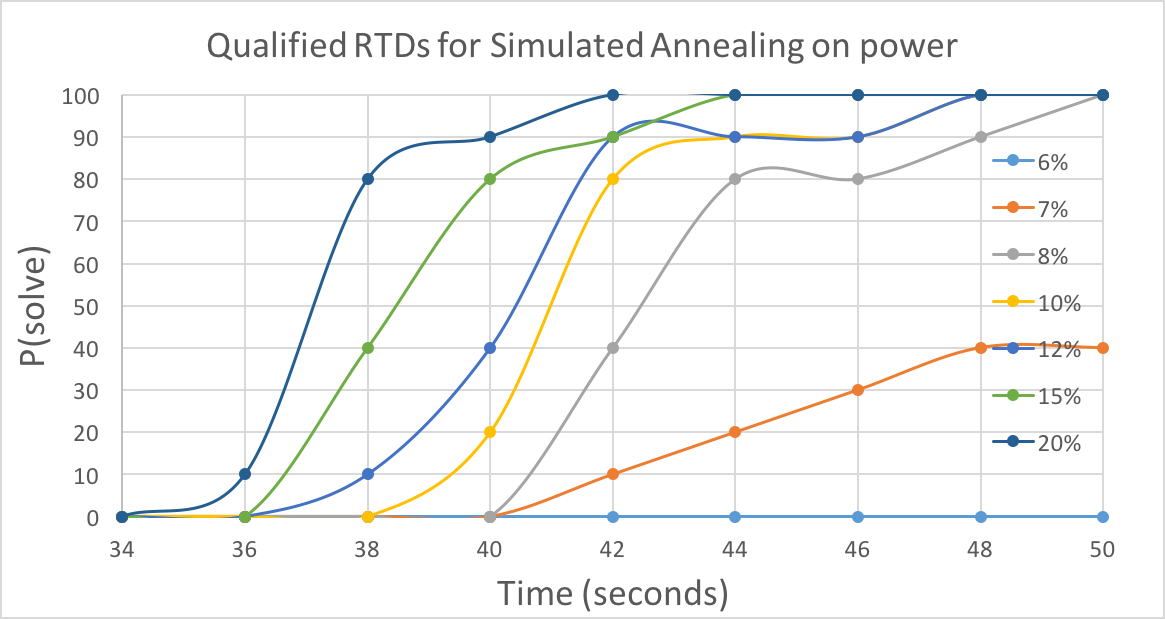
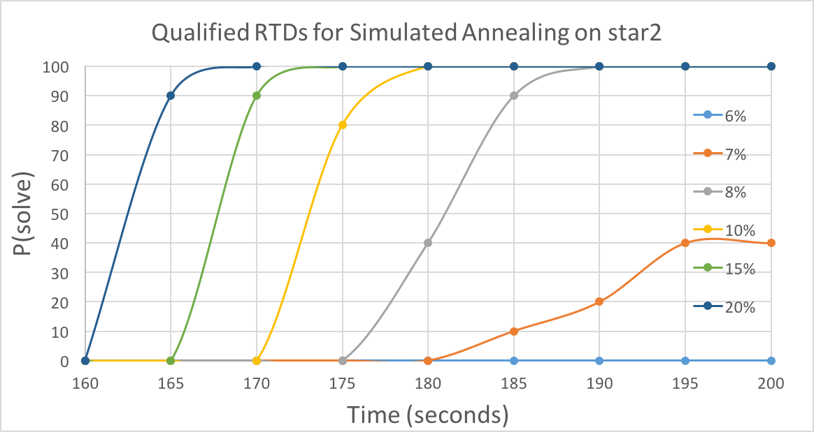
With time increasing, there is a greater probability of reaching specific solution quality. Higher solution qualities require more time. For power graph, there is a boost around 1.1 seconds, indicating most runs obtained a fine solution at this point, though 3% quality is hard to reach for hill climbing algorithm. For star2, the boost is not so obvious compared to the previous one, and 6% quality is rarely reached.
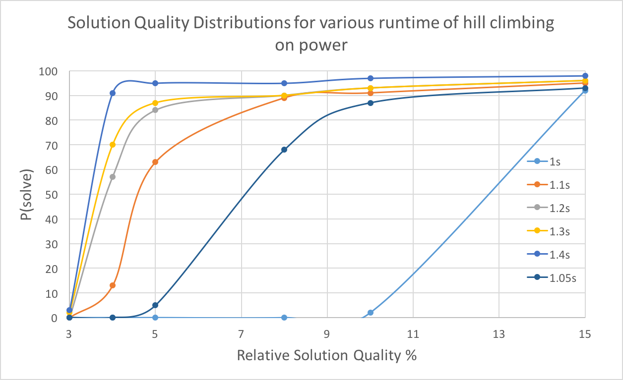
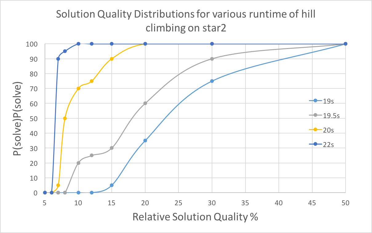
4.3.4 SQD
With less low quality requirement, the running time for hill climbing will decrease. And when quality requirement is the same, longer time will lead to a higher successful probability.
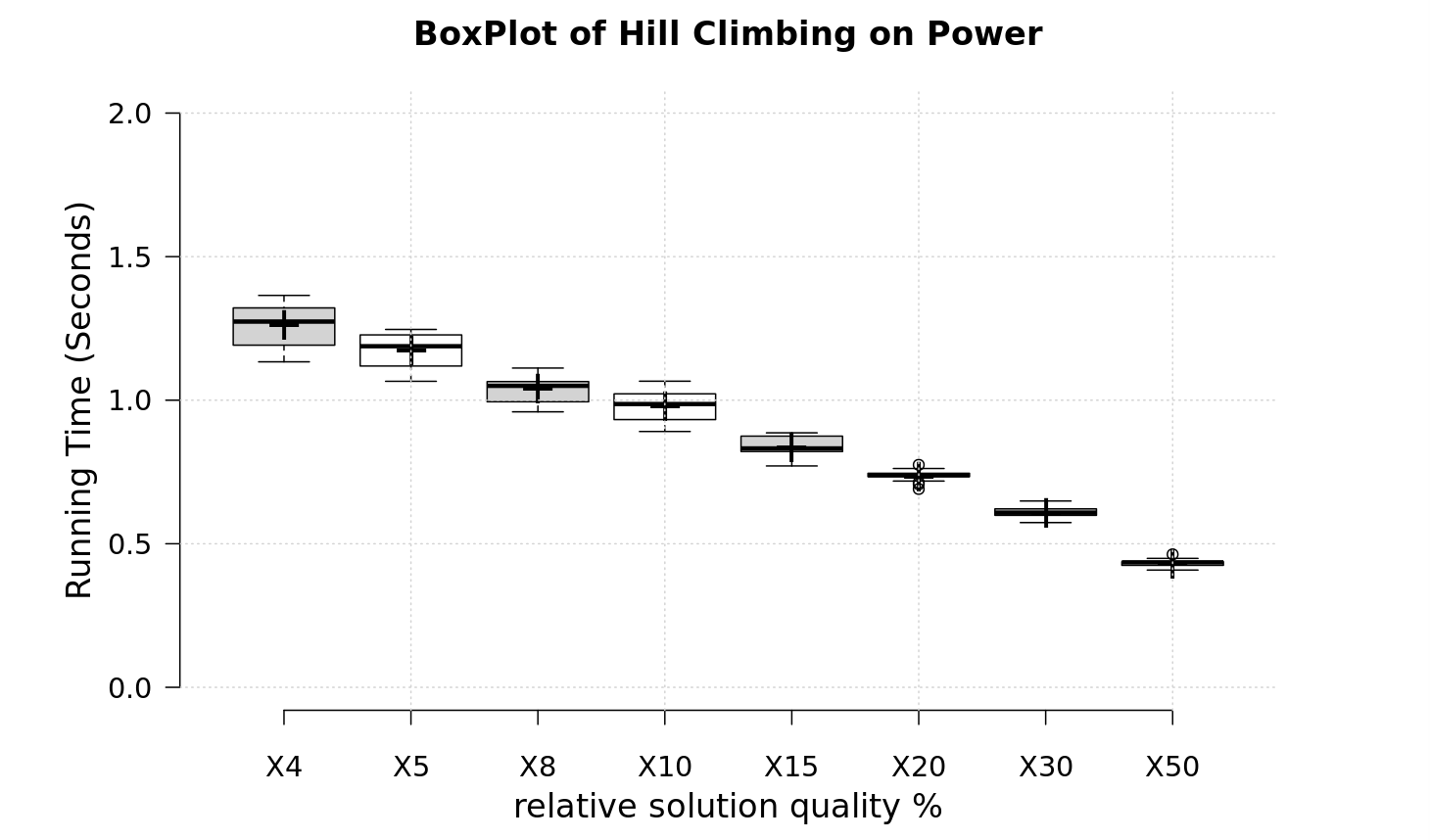
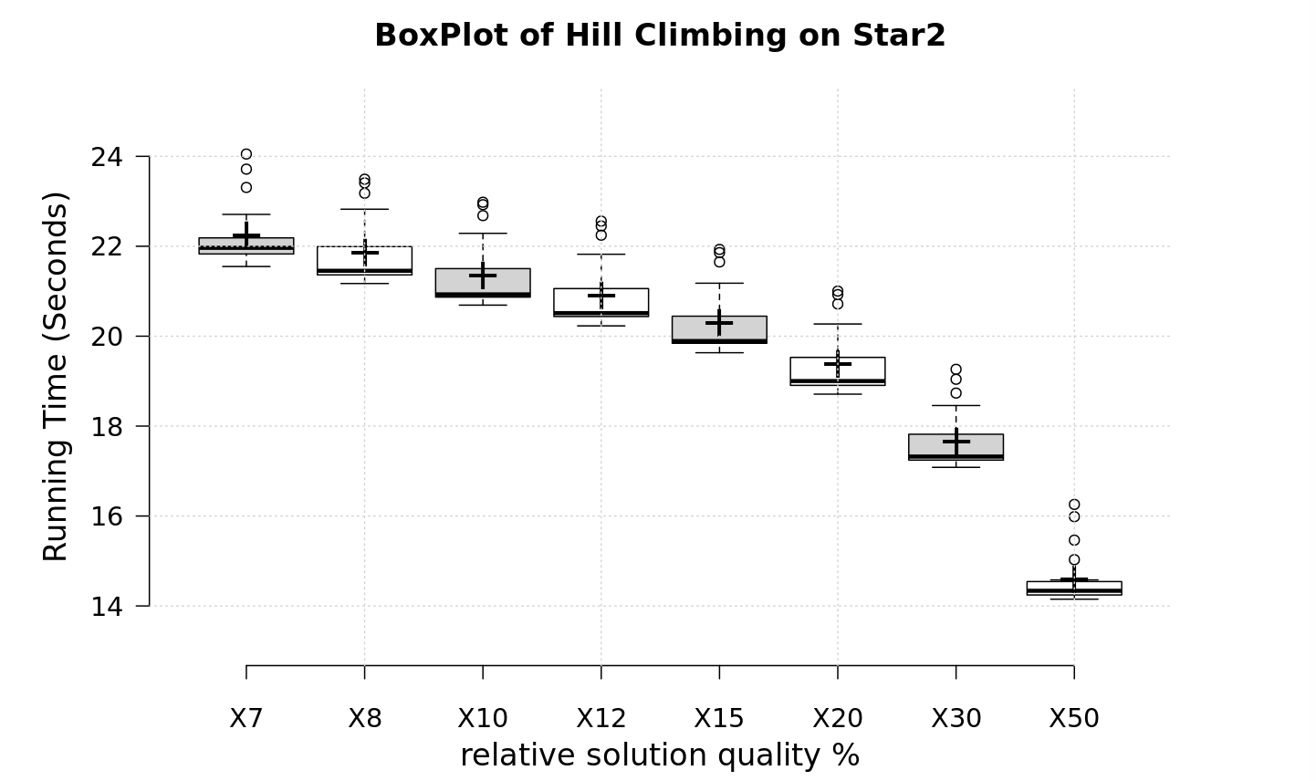
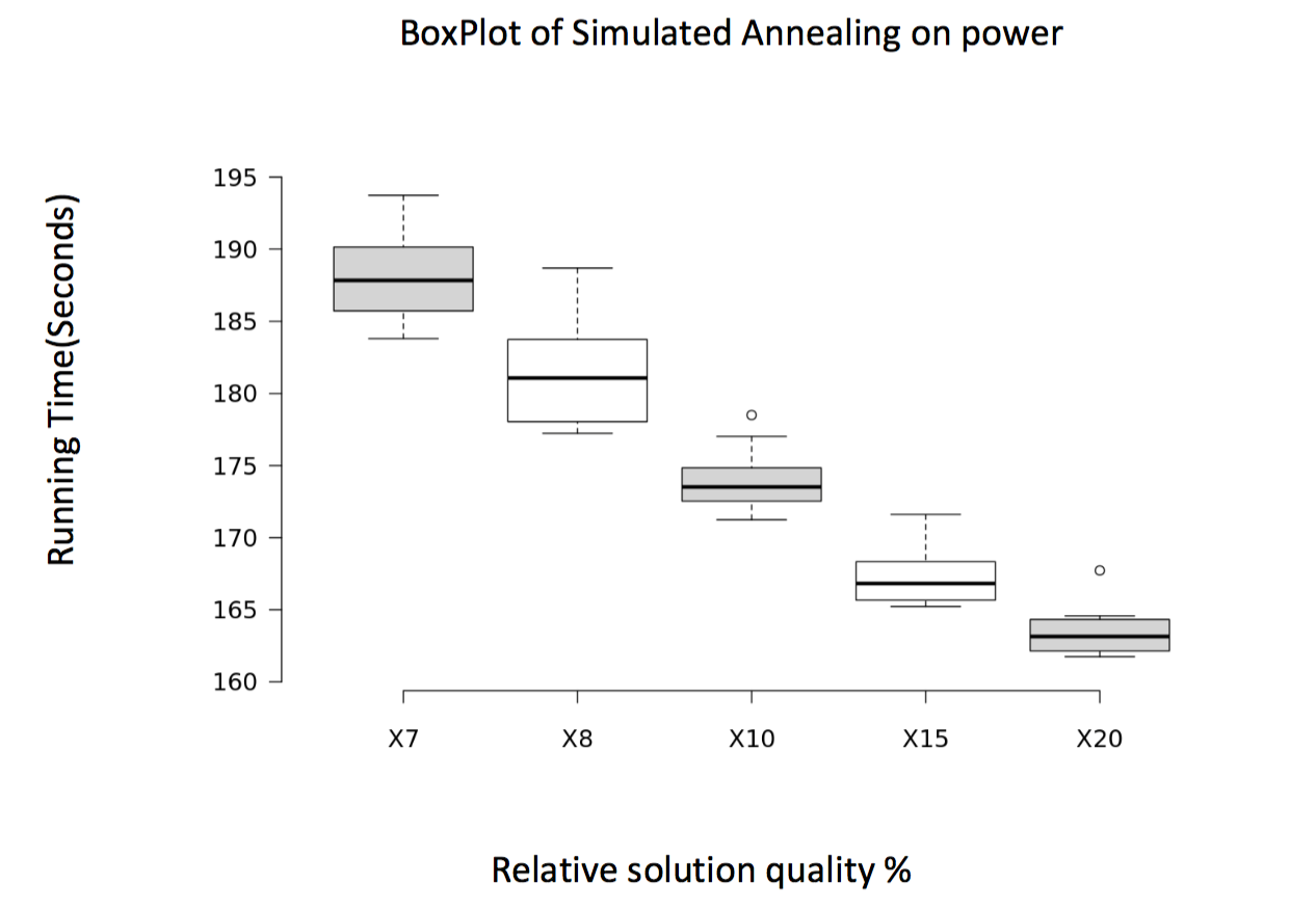
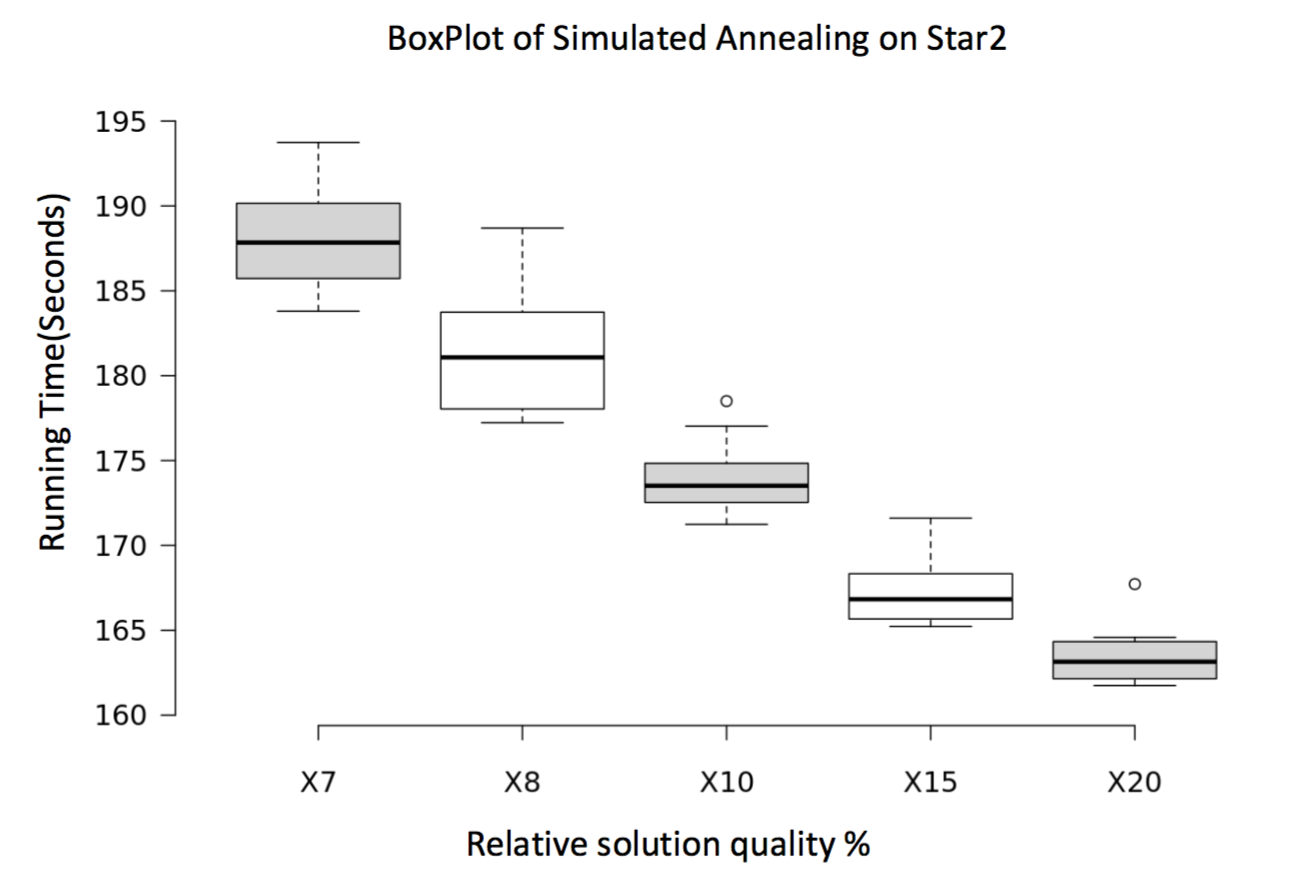
4.3.5 BoxPlots
The decreasing tendency indicates that, with lower quality requirement, the average running time required will be smaller, though some variance may occur. And due to large size of star2, and more nodes with same degree, the random range is greater than that of power, resulting in a larger variance in star2 figure.
5. DISCUSSION
5.1 Branch and bound
The branch and bound algorithm performs well in the test for all samples graphs. Although running time grows exponentially with the increase of graph size (both number of vertex and edges), this algorithm can still give a near-optimal or optimal solution for the Minimum Vertex Cover problem. Furthermore, because of the strategy we chose where every branch either chooses the vertex with most degree or all its neighbors, the near-optimal or optimal solution can be generated quickly (i.e. from the comprehensive table, a considerable solution can be generated within 1 minute for the sample graph with the highest number of edges). The relative error for these graphs lies in a range of 0.00% to 5.84%. The proportional element corresponding to the running time is the number of edges rather than the number of vertex.
The approximation algorithm is used to calculate the lower bound and the solution generated by the approximation algorithm is less than twice the size of the true optimal solution. The lower bound is at least half the size of the true optimal solution and the optimal lower bound should be exactly half the size of the current best solution from the branch and bound algorithm.
5.2 Hill climbing
The hill climbing algorithm also performs well for all test samples, with the largest test graph solved in less than one minute. Errors are relatively controlled, with less than 7% for all test graphs and a few that can reach 0% error. This algorithm is an efficient way to find the minimum vertex cover, when accuracy is not strictly required to lie within a percentage.
5.3 Simulated annealing
The simulated annealing algorithm returns relatively accurate results. By occasionally accepting a worse solution, it runs for a longer time than hill climbing. In exchange, it can escape from local minimas and make another attempt at finding the global minima. However, this random element also deeply affects the data we gathered. Ranging from 0% to 7% in no particular trend, we found no relationship between relative error and input data size.
