Traffic Modeling & Simulation
Group menber: Eric Hein, Xiangyu Liu, Thea Knudsen
Problem description
In this problem we investigate traffic on a section of road in Midtown, Atlanta, specifically the section of Peachtree St between 10th and 14th St. We are interested in predicting the average travel time in this section of road for two different scenarios: when the traffic lights at the intersections are unsynchronized, and when they are synchronized. The goal is to find a way to synchronize the traffic lights in a way that will decrease the average time it takes to travel through this section of road.
In order to predict the traffic, we use a discrete event simulation based on traffic data for the road section in question, collected for the NGSIM project by the Federal Highway Administration. The data was collected between 4:00 and 4:15 pm on November 8, 2006.
To solve this problem, we need a great amount of properties such as the signal timing pattern, the structure of lanes at different parts of Peachtree Street, the feature of vehicles and the drive habit for different drivers. To analyze these, here’s some more detailed information about our project.
We can use 5 Ws to start the description.
WHEN: Our simulation model focuses on the afternoon commute time at which the original data was caught, between 4:00 p.m. and 4:15 p.m.
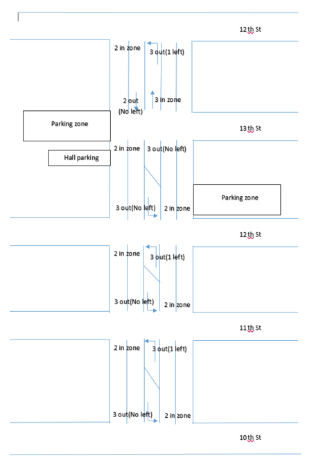
WHERE: The model takes place in 10th to 14th street and the data is generated from that point. We decide to use the map below from the google map which has something different compared with the data.
WHO: The main component in the model is the vehicles on the road. This component may be affected by many aspects. We made some assumption to simplify some ignorable parameter.
WHAT: it means what to do with the model. The input should be the distribution of vehicles based on the data. This simulation model focus on vehicles’ status.
Record of the travel time for every vehicle
HOW: there are two different cases we will consider separately, synchronized and unsynchronized traffic signals.
To sum, we plan to use the given data to draw a discrete event simulation to compute the travel time for each vehicles from different entrances to different exits at 4:00 p.m. to 4:15p.m. on the Peachtree Street from 10th to 14th street.
The traffic data and signal timing pattern come from project file and the lanes information for each intersection comes from google map.
Desired Output
Record of the travel time for every vehicle
Recod of the travel time at main lanes (Northbound and Southbound on the Peachtree St.)
Street Map
5 intersections (4 signal lights, 13th St doesn’t have one)
5 lanes (10th to 13th has 2 straight lanes and 1/2 left turn lane, 13th to 14th has 2 straight lanes southbound and 2 straight lanes and 1 left lane northbound)
11 entrances and exits
Conceptual model
The road traffic is modeled as follows: A vehicle arrives at an entry zone according to a Poisson process. The arrival rate at each entry zone is different and is based on the NGSIM data. As a vehicle arrives, it will continue towards the next intersection. If the light at the intersection is red, the vehicle will get in the queue to cross the intersection and wait until the light turns green. If the light is green or yellow, there is no queue and no wait time. The next event is that the vehicle either crosses the intersection or exits the simulation domain. If it crosses the intersection, it will get in the queue for the next intersection.
Data Extraction and Input Analysis
Arrival rates
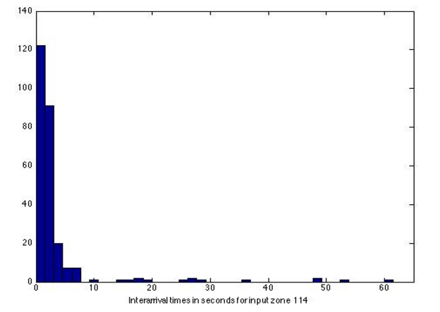
To find the distribution of the interarrival times for each input zone, all interarrival times for each zone were extracted from the NGSIM data set. For each input zone, the set of interarrival times were fitted to an exponential distribution. It is a common assumption to make that interarrival times are identical and independent exponentially distributed. The interarrival times for input zone 114, which contains the southbound lanes entering the intersection of Peachtree and 14th street, are shown in the histogram below.
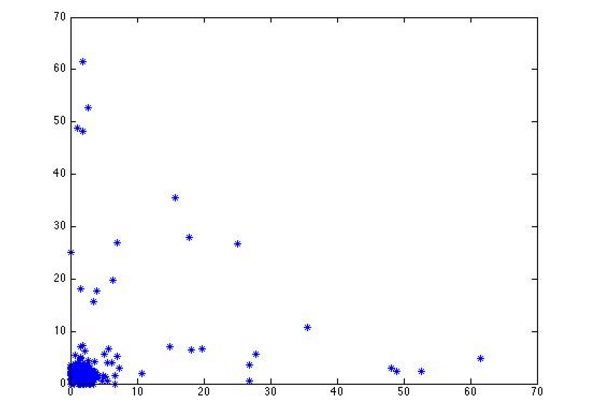
Observe that the data seems to be following an exponential distribution for the smaller inter- arrival times. However, there are some larger interarrival times that do not fit well in an exponential model. This is likely due to waves of traffic arriving from intersections north of 14th street. The same phenomena is seen in the interarrival times for the northbound lanes entering Peachtree/10th street. To check for independence, pairs of interarrival times (ti,ti+1) were plotted against each other. The scatter plot below shows that there is no significant correlation between subsequent arrival times.
Despite the larger interarrival times in the data set, we choose to model interarrival times exponentially. The exponential distribution fitting was done using MATLAB’s fitdist function, which fits a data set to the given type of probability distribution using maximum likelihood estimators to estimate the parameters. In this case the parameter is the arrival rate, which is the inverse of the mean interarrival time.
Routing Probabilities
In this simulation, a car will be randomly assigned to an exit zone when arriving at an input zone based on a probability model. These probabilities were extracted from the NGSIM data set by looking at all the different input zone-output zone pairs in the model, and counting how many cars followed that particular routing. Then, for each input zone, the fraction of cars exiting at a particular output zone was calculated, and this was used as the probability of getting assigned to that output zone in the simulation.
Traffic Light Timings
The timings for each traffic light were also provided by the NGSIM data set. We made some minor adjustments to the timings such that for each light, the red-green-yellow cycle added up to the same total time of 100 seconds. Within each intersection, the start of the cycle for each individual light was adjusted so that together they mimic a real intersection, e.g., north- and southbound lanes have a red light while east- and westbound lanes have a green light.
Random Number Generator
For generating random numbers for interarrival times, routing probabilities and signal initialization, we used the rand() function in the C++ std library, which is a thoroughly tested linear congruential generator. For the interarrival times, the random number generated was used to find a uniform(0,1) number u. Then, using the inverse transform theorem, interarrival times X were sampled as x = F’(u), where F(x) = 1-e^(-rx)
is the cumulative distribution function (CDF) for an exponential distribution with arrival rate r.
Assumptions
When constructing a conceptual model the data set used for this simulation is quite extensive, so a more detailed model could certainly be developed, but because time constraints we are making the following assumptions:
Reaction time: We assume that each vehicle in line has a constant reaction time (delay) from the time a vehicle is allowed to move and until it actually starts moving. The average drive delay we extracted from the data is 1.9 sec.
Acceleration: Since the acceleration time for vehicles from start to average velocity is very short, we exclude acceleration in cars from standstill, assuming that all vehicles will start and stop directly.
Velocity: From the data it tells that the velocity distribution for a certain time has a dominant intersection. So we assume that all vehicles share the same velocity in the model.
Exit zones: Assume there is always room to exit the simulation in a zone because for a general situation lanes can hardly be full.
Determination of input and output zones: Vehicles arrive input zones based on the distribution from the data, and determind the output zones after they arrive. And the proper lanes will be decided from input zones to output zones.
Drivers behavior: We assume that all driver will choose the lane with shortest queue unless he is turning on the next light (with a “buffer”; will not change lane if the queue in the other lane is only a little bit shorter).
Choose turning lane: We assume that the car gets into the turning lane in the section just before the turn.
Driver types: We also assume that all drivers follow the same driving pattern based on where their end zone is, in other words, no different driver types.
Other general assumptions: No bad weather, No traffic accident, No crossing people, etc.
Simplifications
To make the simulation program easier to implement, we make some simplifications to the model.
Vehicle size: We assume that all vehicles are the same size. To account for larger vehicles (trucks) taking up more space on the road, the arrival rate can be adjusted accordingly. This simplifies the implementation of the simulation model significantly.
Stop Distance: We assume the distance between stopped vehicles is constant since it can be added to verify how many vehicles can a lane contain.
Intersection: Each lanes is designed to have its own crossing event schedule (in other words, it has an intersection zone for itself), so that we simplify our model that vehicles cross the intersection one at a time.
Lane changing: Since we assume vehicles will choose turning lane in the intsection, we make a simplification that vehicles won’t change lanes in the sections.
Filtering zones: based on the data, there are some input and output zones that have a very low rate for vehicles entering and exiting (the Google Map shows that these zones represent parking lots). We filter these zones because it hardly affects the distribution and hurts the simulation.
Code description
Simulation Executive
There are several ways to implement a discrete event simulation. We have chosen to use an event oriented world view, which means that simulation program is built with a focus on a series of events happening rather than following entities through the simulation process. The simulator was written in C++. No outside software packages were used, besides several container classes from the C++ Standard Template Library (STL). The simulation executive uses a priority queue to keep events sorted by timestamp. The future event list (FEL) is implemented as an STL priority_queue. The main loop executes one event from the queue at a time, halting only when it reaches a special stop event.
Software Architecture
Detailed documentation of the simulation code has been generated using doxygen. The documentation is located in the attached source distribution in the folder doc/html. Open the file hierarchy.html in a web browser to view.
The application code is heavily object oriented to separate the behavior of each entity into its own class. The majority of the classes fall into two categories, State and Events. All Events inherit from the event class, so that the executive can use polymorphism store them in the priority queue and call the process() method on each one. The other folder contains classes that represent the state of the system, such as the color of each traffic light, the line of cars waiting at an intersection, or the destination zone of a vehicle.
State classes typically have an event in the queue at all times to control the next update of the entity. For example, the traffic light constructor schedules the first color change event. When this event is processed, it changes the color of the light and schedules the next color change based on the traffic light timing parameters. Similarly, every arrival of a vehicle at an input zone schedules the next arrival at that zone based on a probability distribution. Each lane schedules intersection crossing events for its own cars, taking into account the color and timing of the traffic light to decide when the next crossing will occur. If no vehicles are in a lane, the next crossing event will be scheduled as soon as a car enters the lane.
Testing
For testing, we simulated a single traffic stop on a one-way road. Cars enter at a constant rate from the south, cross an intersection governed by a traffic signal, and continue to the north. Once this was working, we gradually added more features, testing as we went. An important part of simulator verification was the liberal use of logging functions to print the timestamp and an informational message whenever an event executed. With these messages in place, we could watch as the simulation progressed and gain insight into the correct operation of the simulator.
Initialization
In order to recreate the Peachtree network in our simulator, many lanes, traffic lights, and input/output zones need to be created. The Intersection class provides several helpful methods for doing this in an orderly manner. The main function initializes the network in the following manner. First, an intersection is created. Then, lanes are attached to the intersection in each direction. Traffic lights are associated with each lane during this step. Each lane has two traffic lights, one for left turns, and another for going straight or making a right turn. To emulate a left-turn only lane, a “dummy” light that is always red is inserted in place of the straight light. Placing a dummy light in the left turn light produces a lane that can only go straight or turn right. Finally, lanes are connected between intersections. This step determines which directions vehicles can go from each lane. Before the simulation begins, each lane traverses all possible paths to discover which output zones are reachable from itself. This routing table is stored and used by vehicles as they traverse the system to decide when to lane change into a turning lane.
Output
For each vehicle that reaches an output zone, the simulator outputs the source zone, destination zone, and the time the vehicle spent in the simulation. For debugging purposes, the simulator This can be used to calculate the average time a car uses to pass through the domain, which is what we wish to predict for both the unsynchronized and the synchronized case.
Simulation results and output analysis
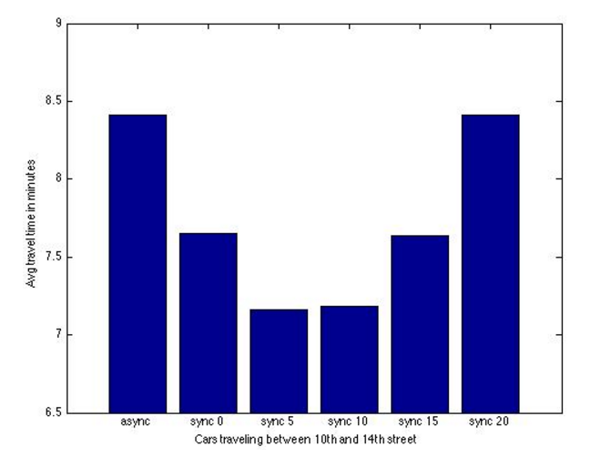
The purpose of this simulation was to compare traffic flow on a simulated portion of road when using unsynchronised versus synchronised traffic light timings. Each intersection had a traffic light cycle of 100 seconds. For the unsynchronized simulation runs, each intersection started the traffic light cycle at a random time in the cycle, independent of the other intersections. Let t(cyc) describe where in the cycle a traffic light is at the beginning of the simulation. In the synchronized runs, the traffic lights at the intersection of Peachtree and 14th street started at the beginning of the timings cycle, t(cyc)=0. When traveling south, each intersection had a delay in t(cyc) of x seconds compared to the previous intersections, for x = {0, 5, 10, 15, 20}. Then, for each synchronization, we looked at the difference between the average simulated travel time per car for the unsynchronized and the synchronized runs. Each instance was run 30 times, and the average over these 30 runs was used for the comparisons of instances.
Results
We looked the travel times both for all cars in the simulation, and for only those that traveled through the entire simulation domain, i.e. from 10th to 14th street or from 14th to 10th street.
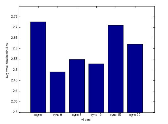
Plots of the average travel times are shown below:
For all cars (top), it looks like delays of 0, 5 and 10 seconds all give shorter travel times. For the north/south traveling cars we also see an improvement for a 15 second delay. This was confirmed with 95% confidence when performing a paired t-test on the average difference d between the average travel times for the unsynchronised and synchronised systems.
Conclusion
After careful modeling, input analysis, and software design, we successfully simulated traffic flow through several intersections on Peactree Street. The results gathered from this simulation show that traffic light synchronization is almost always better than unsynchronized operation. Specifially, an offset of 5 seconds between adjacent lights dramatically improved travel time for cars traveling north and south on Peachtree Street.
